Explore

A one-click profile of any table: per-column distribution, null ratios, distinct counts, sample values. Think pandas-profiling but inline and SQL-agnostic.

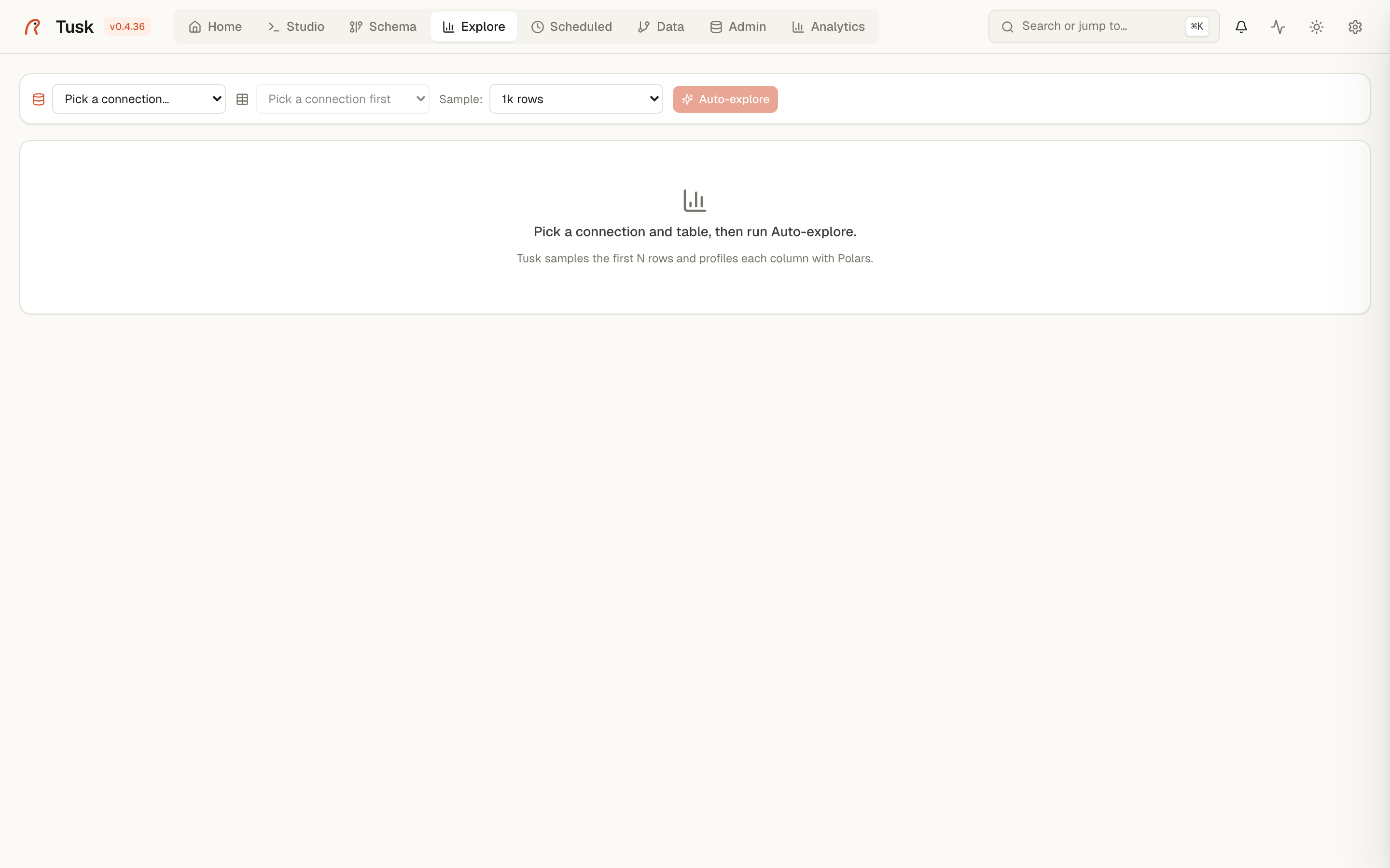
Explore — auto-profile of a table with per-column stats and histograms.

How it works

Pick a connection + table + sample size. Tusk runs a series of cheap SELECT queries against your data (with LIMIT and TABLESAMPLE where applicable to keep cost bounded), aggregates the results client-side, and renders one card per column.

Example flow from the screenshot:

• Connection: <your postgres> · <schema>
• Table: public.regions
• Sample size: 1k rows (other options: 5k, 10k, 100k, full table)
• Click Auto-explore → ~2-5 seconds later you have a profile.

Top of the page shows the header tile: rows sampled, total columns, table identifier.

Per-column cards

Each card is sized by column type — strings render their top values + frequency, numerics render min/max/mean/Σ + a histogram, booleans render a bar pair, dates render a year-month timeline.

A typical card:

┌─────────────────────────────────────────────────────┐
│ T  level   int64           100% complete  4 distinct │
│ ─────────────────────────────────────────────────────│
│ MIN     MAX      MEAN    Σ                          │
│  4       8       7.856   0.4187                     │
│                                                     │
│ 8  ████████████████████████████████████████  8,748  │
│ 7  ████████                                  1,112  │
│ 6  ▌                                            116 │
│ 4  ▏                                             24 │
└─────────────────────────────────────────────────────┘

The strip below the header has two stats: % complete (1 − null ratio) and distinct value count. A red bar with 100% nulls is a quick visual flag that the column is empty in your sample.

What the cards adapt to

Column shape	Card style
Categorical (string, < 50 distinct)	Top-N frequency bars
Numeric (int / float / numeric)	Min/max/mean, total, histogram
Boolean	Two bars, true vs false
Date / timestamp	Year-month timeline
High-cardinality string (≥ 50 distinct)	Just the first 10 sample values + the distinct count
All-null	Red "100% null" banner, no further detail

When to use it

• First contact with a table — you want to know what's actually in it before writing a query.
• Data quality spot-check — sudden spike in nulls or distinct-count drift suggests an upstream regression.
• Picking a join key — the distinct-count + null-ratio + sample-value combo tells you whether a column is safe to join on.
• Pre-flight for a dashboard widget — confirm the column shape before wiring it into a Top-N or Funnel widget in Analytics.

When NOT to use it

• For business metrics — Explore samples your data; numeric aggregates are approximate. Use Studio for exact aggregates.
• For tables you query every day — it's exploratory. Saved queries + dashboards are the right answer for recurring questions.

Performance notes

• Sample size capped at 100k rows; beyond that, the cost-vs-signal trade-off goes the wrong way.
• For tables > 1M rows, prefer 5k rows sample — the distributions stabilize fast.
• All Explore queries respect the connection's statement_timeout and the per-request RequestTimeoutMiddleware budget. If they take too long, the page returns a 504 cleanly rather than hanging.

Related

• schema.md — for the model view; Explore is the data view.
• studio.md — the "Query in Studio" button on each card opens an editor with a SELECT <col>, COUNT(*) template.

Spatial columns

On a PostGIS table the profile starts with its geometry columns: type, SRID, spatial index, invalid geometries in the sample and the extent — the same checks as the Admin Spatial card, for the table in front of you.

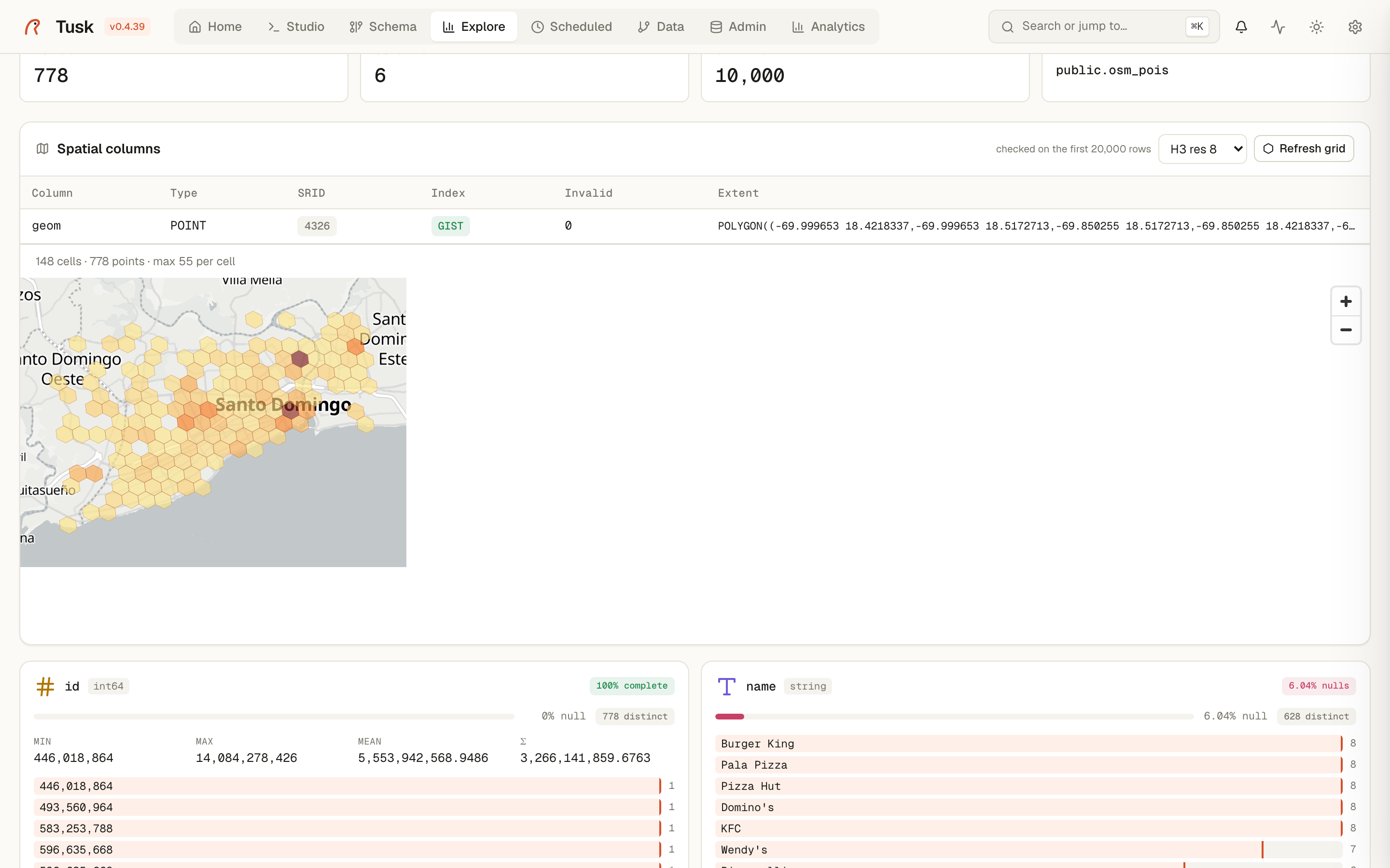
Density grid aggregates the table's points (or the centroids of its polygons, or a lat/lon pair) into H3 hexagons at the resolution you pick (5 = country blocks, 10 = city blocks) and draws them on a map with the count per cell. It runs in Python on up to 200,000 rows; no h3-pg extension is needed.